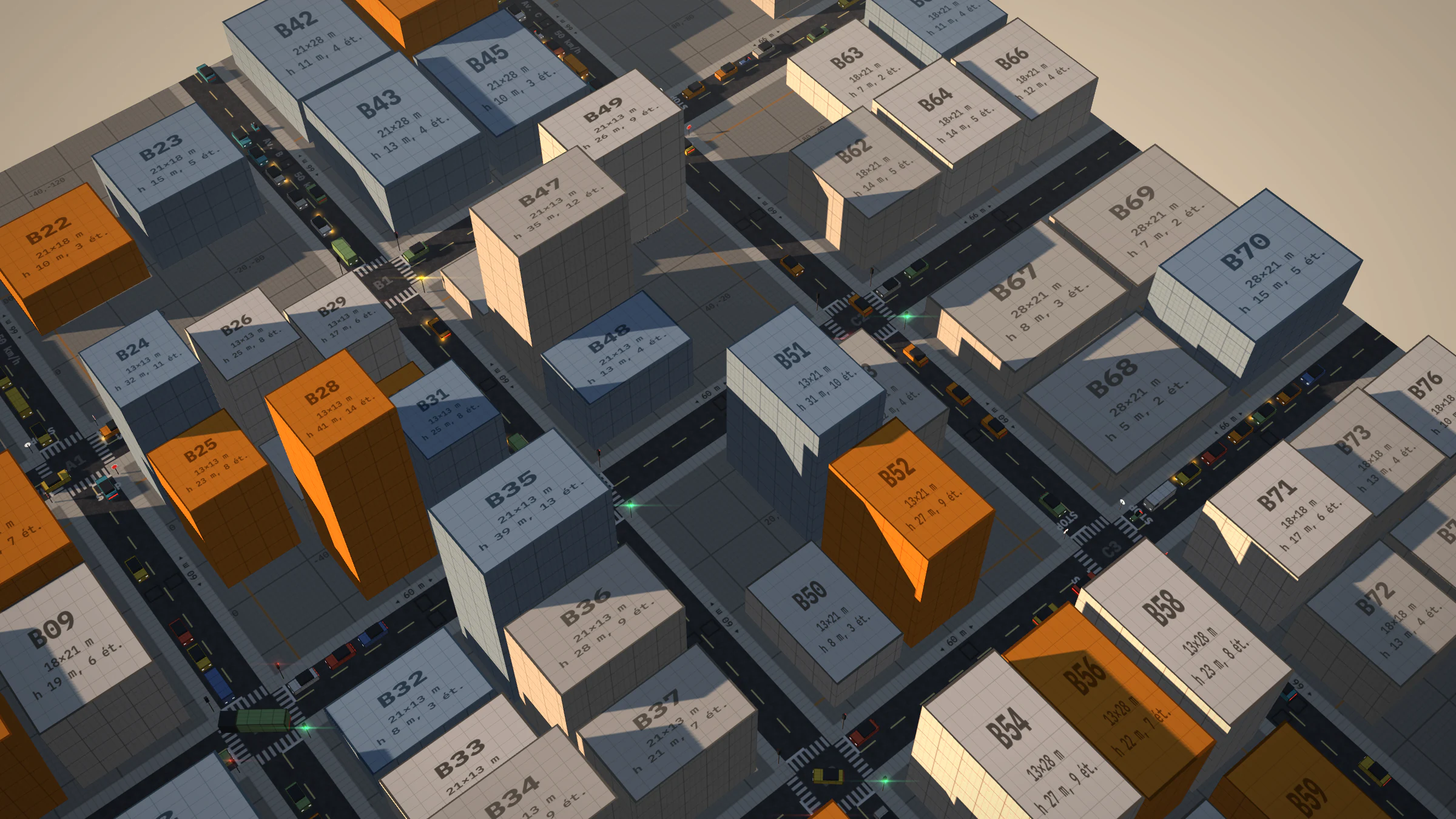
Lab · Simulation · In progress
Trafic
A real-time microscopic traffic simulator in JavaScript, rendered with three.js. Every vehicle has its own driving model, route and junction bookings. The engine is independent of rendering and validated under Node by a twenty-scenario bench; networks are described in JSON; one vehicle can be driven.
- Engine
- JavaScript
- Rendering
- three.js r128
- Bench
- 20 scenarios
- Roadmap
- 28 / 50
- Reading
- 16 min
Trafic computes every vehicle individually, at a fixed 1/30 s step, and three.js displays it in the browser. The demo network is a 3 × 3 grid of junctions; the engine also reads other networks, described in JSON.
The roadmap’s goal: approach the realism of the reference simulators (SUMO, PTV Vissim, Aimsun) while staying real-time. Development follows fifty features ordered by size and dependencies, one per commit; each is measured by a headless test bench and documented by a figure generated by the engine. This page describes the state at #28.
Log 01 / 10
Engine core
Car-following model, fixed step, seeded randomness, headless test bench, spatial index.
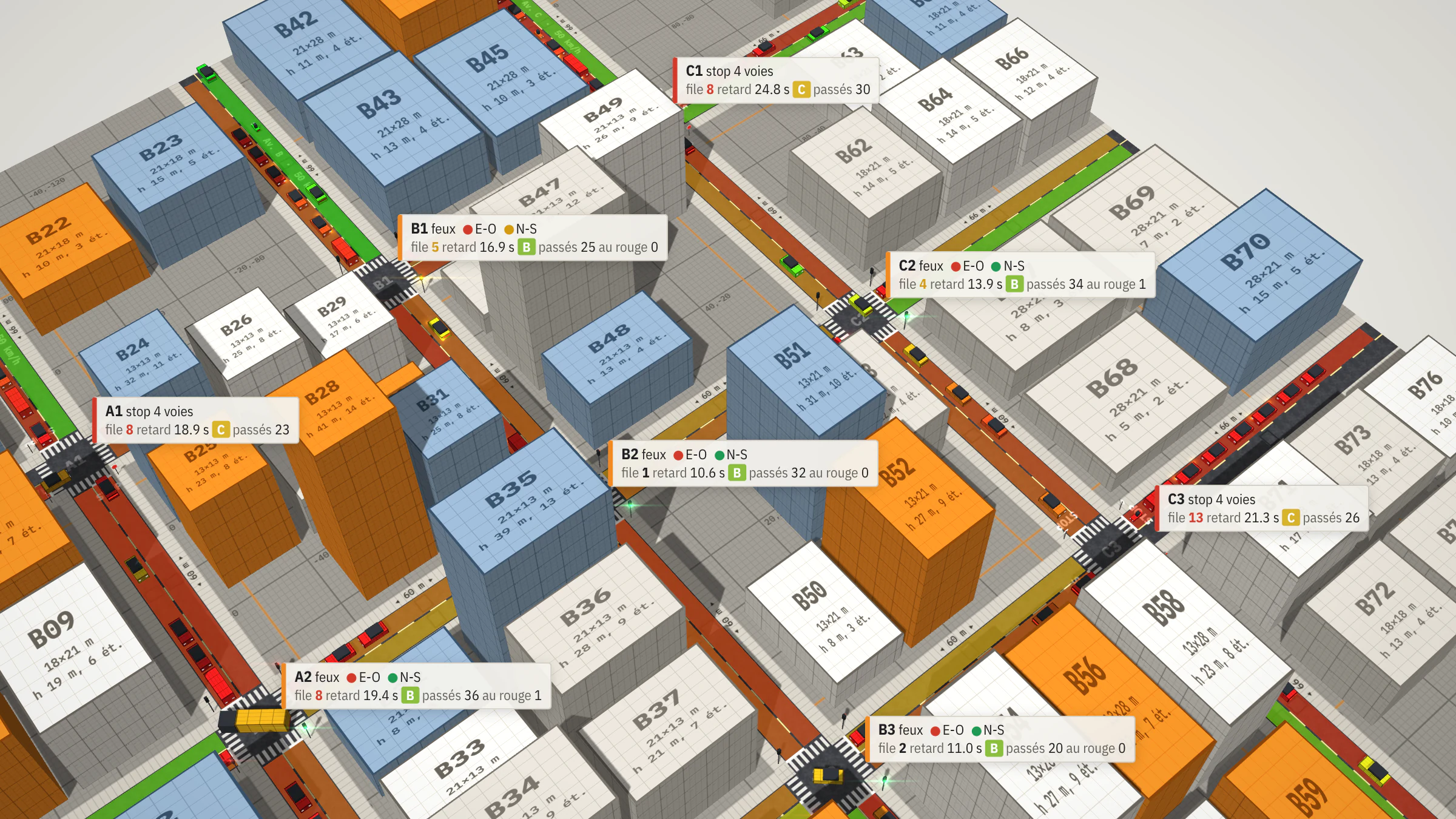
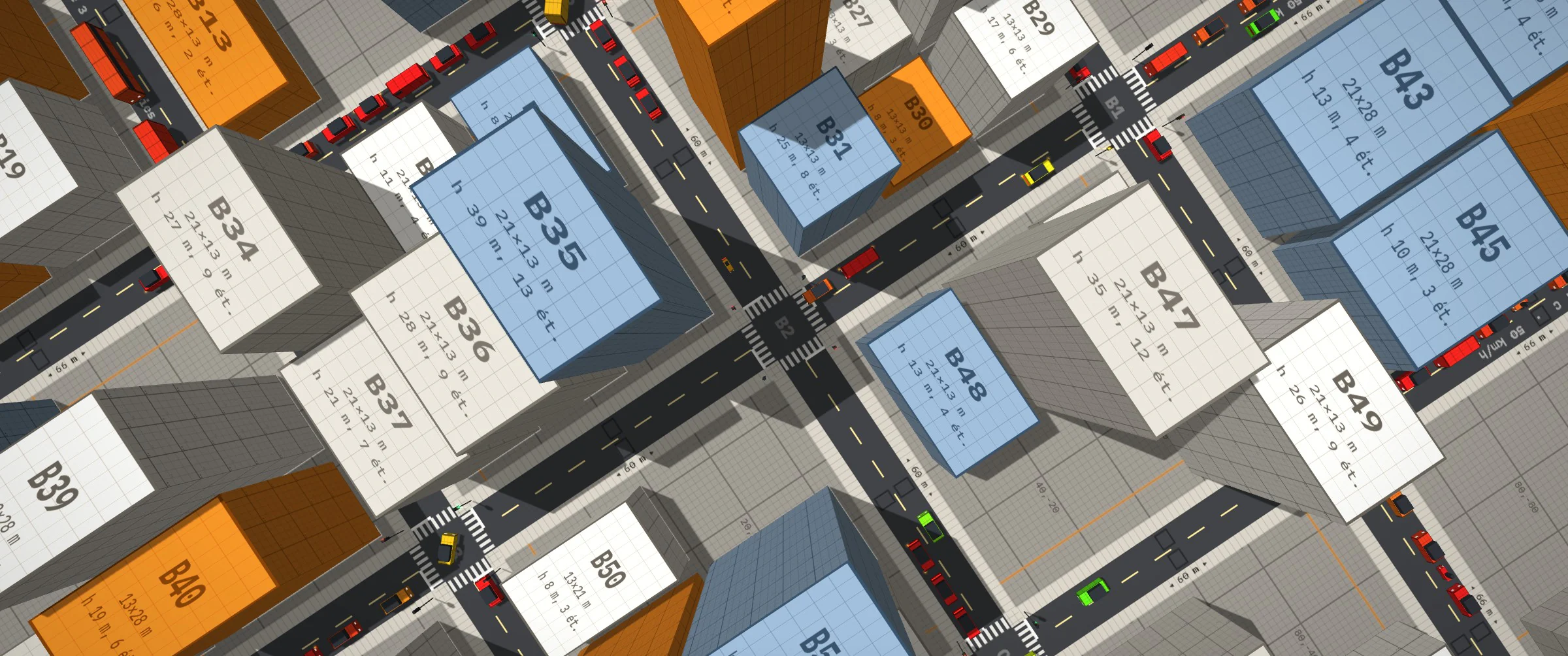
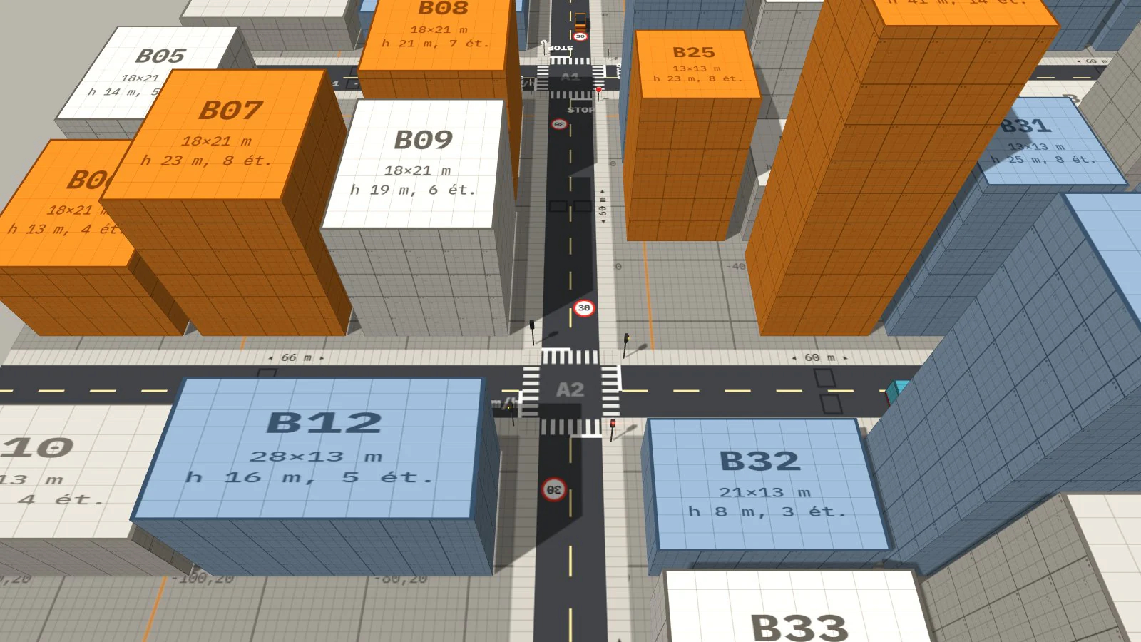
Demo network: a 3 × 3 grid of junctions 60 m apart, one lane each way, twelve entry-exits. Every vehicle follows the IDM: its acceleration depends on the gap and relative speed to the first obstacle on its path, a vehicle, a stop line or a vehicle already in the junction. It books the junction before entering it. The simulation step is fixed and decoupled from display; at start-up, 25 s of traffic are pre-simulated.
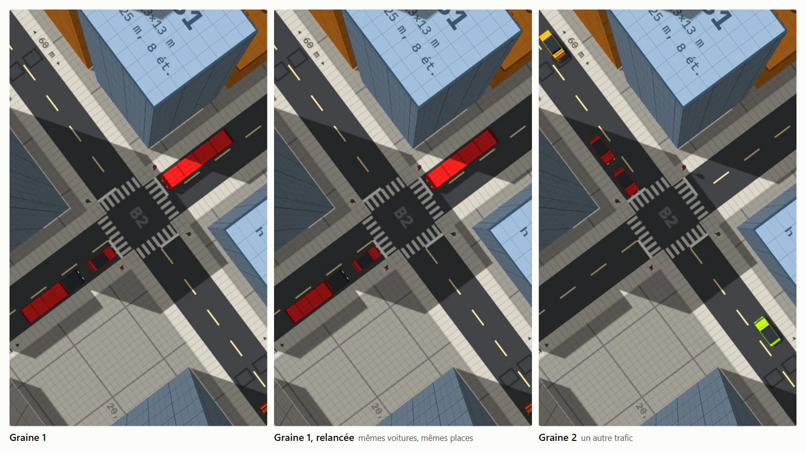
Determinism: all randomness in the traffic goes through a seeded generator (mulberry32) instead of Math.random: spawns, destinations, driver parameters, colours. Same seed, same trajectories. The seed is passed in the URL (?seed=42).
Test bench: npm run bench runs the simulation headless under Node on twenty reference scenarios, six seeds each, and compares the indicators’ means against a reference; a difference is only flagged beyond three standard errors, since the variance between seeds is 5 to 15%. An exact fingerprint of the final state validates refactors that should change nothing, bit for bit. Seed 1 runs as three simultaneous copies: fingerprints compared for determinism, best time kept for the step cost.
- 1/30 s
- Fixed simulation step; rendering interpolates between the last two steps.
- 20 × 6
- Reference scenarios × seeds per scenario.
- 0.20 ms
- Cost of one step at saturation, about 170 vehicles.
Spatial index: a grid of 50 m cells rebuilt at every step (only the 3 × 3 neighbouring cells are read), then a bounding-box test on the 22 points sampled ahead of the vehicle. Both filters are exact: fingerprints unchanged. At saturation, a step goes from 0.25-0.29 ms to 0.20 ms; the gain is mainly for large networks, beyond the current 400-vehicle limit.
Log 02 / 10
Driver model
Randomly drawn profiles, amber decision, reaction time and anticipation (HDM).
Three profiles: cautious (25%), normal (55%), hurried (20%). Each driver draws their parameters around their profile’s values, with an 8% relative standard deviation capped at ±2σ. Effect at saturation compared with identical drivers: exits −4%, average speed −6%.
| Parameter | Cautious | Normal | Hurried |
|---|---|---|---|
| Max acceleration | 1.7 m/s² | 2.3 m/s² | 2.9 m/s² |
| Comfortable braking | 2.0 m/s² | 2.6 m/s² | 3.2 m/s² |
| Time headway | 1.1 s | 0.8 s | 0.6 s |
| Minimum gap | 2 m | 1.8 m | 1.5 m |
| Desired speed | 86% of the limit | 95% | 108% |
| Reaction time | 0.75 s | 0.6 s | 0.5 s |
| Lateness accepted on red | 0 s | 0.4 s | 1 s |
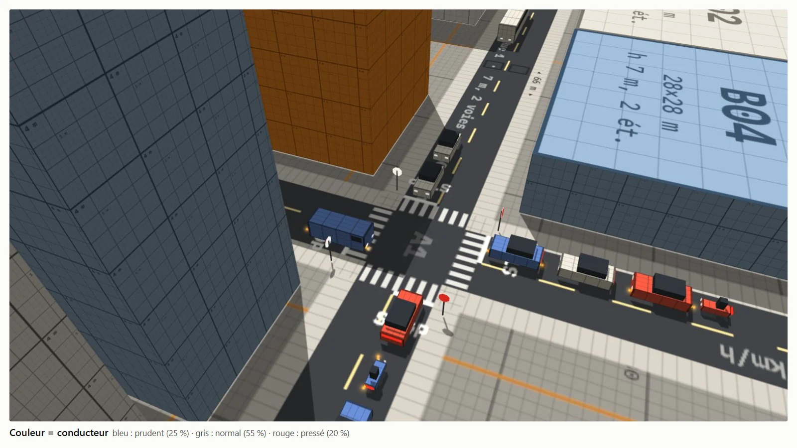
Dilemma zone: when the amber comes on, each driver draws their decision once, from their time to the line, on a logistic curve fitted to Zegeer and Deen (1978): 10% stop at 2.5 s and 90% at 5.5 s for a normal driver, shifted by ±0.5 s depending on the profile. They go if stopping requires more than 4.5 m/s², and give up if they cannot cross the line before their accepted lateness on red runs out. Measured: 0.5 to 0.6% of crossings during the all-red.

Human Driver Model, on by default: each driver applies the decision taken one reaction time earlier (0.5 to 0.75 s), anticipating their position when it takes effect; they estimate distances to ±10% and the closing speed with an error correlated over 20 s; they react to the most constraining of the vehicles visible ahead. Anticipation starts from the accelerations already decided, not from a constant speed: 1 to 2‰ of harsh braking. Parameters were refitted to keep a saturation flow of 1,803 ± 34 veh/h. A box in the panel switches back to the plain IDM.

Log 03 / 10
Junctions and signals
Five junction regimes, gap acceptance, three signal controls.
| Regime | Rule |
|---|---|
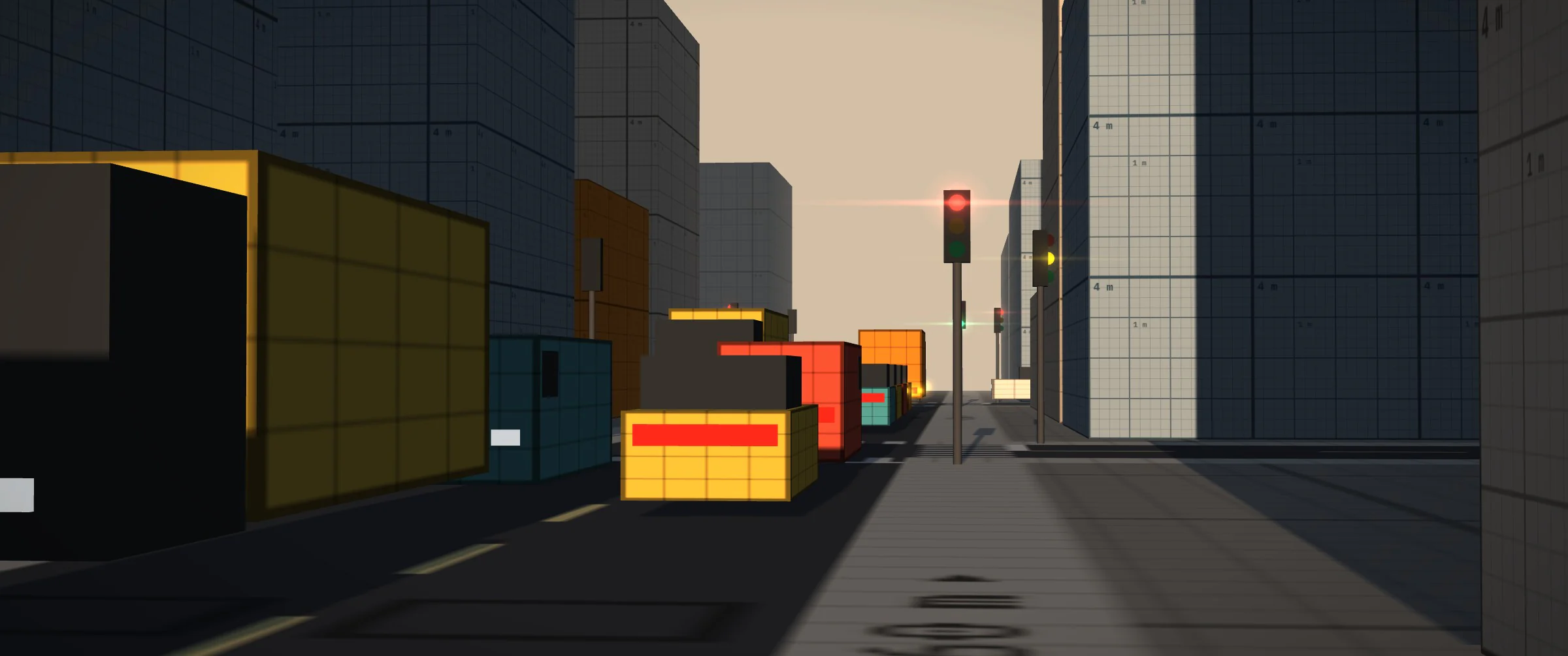
| Traffic signals | Green, 3 s amber, 1.5 s all-red, alternating between the east-west and north-south axes. |
| All-way stop | Full stop required, then first come, first served. |
| Stop on the minor road | Stop, then wait for a big enough gap in the major road’s traffic. |
| Yield | Approach at 16 km/h, pull in if the gap is enough. |
| Priority to the right | Everyone gives way to the vehicle coming from their right. |
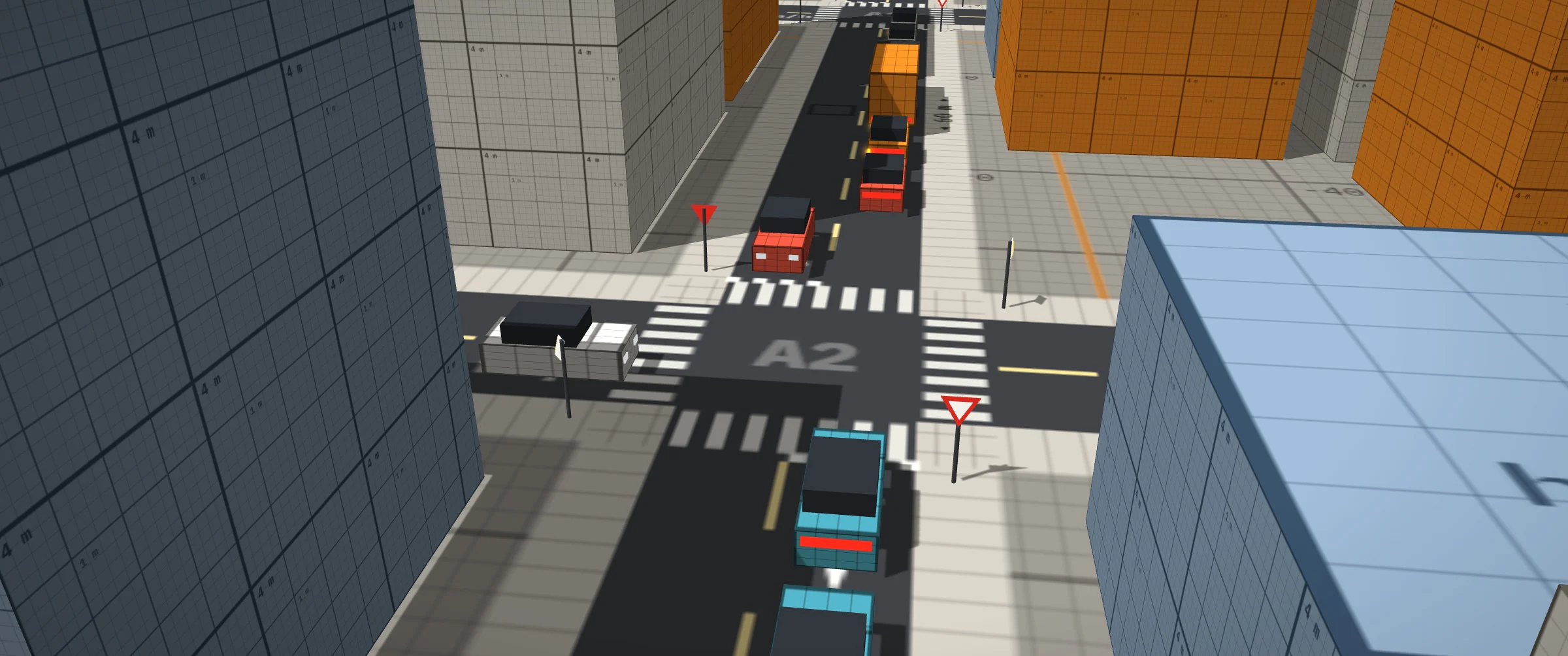
Gap acceptance: a driver who has to give way estimates the arrival of the next priority vehicle whose path crosses or merges with theirs, up to two segments upstream and assuming firm acceleration. They only pull in if the gap exceeds the HCM critical gap: from the minor road, 6.2 s right, 6.5 s straight, 7.1 s left; from the major road, 4.1 s left; all × √(T / 1.1) according to their time headway T. Conflicts are computed on the turning curves.
Actuated signals: detection over the 35 m upstream of the stop lines, phase call by a vehicle on red, 6 s minimum green, extended while vehicles keep arriving, ended after 2 s without an arrival or 30 s after the opposing call. At equal demand against the fixed-time green wave: waiting −7%, exits +4%.
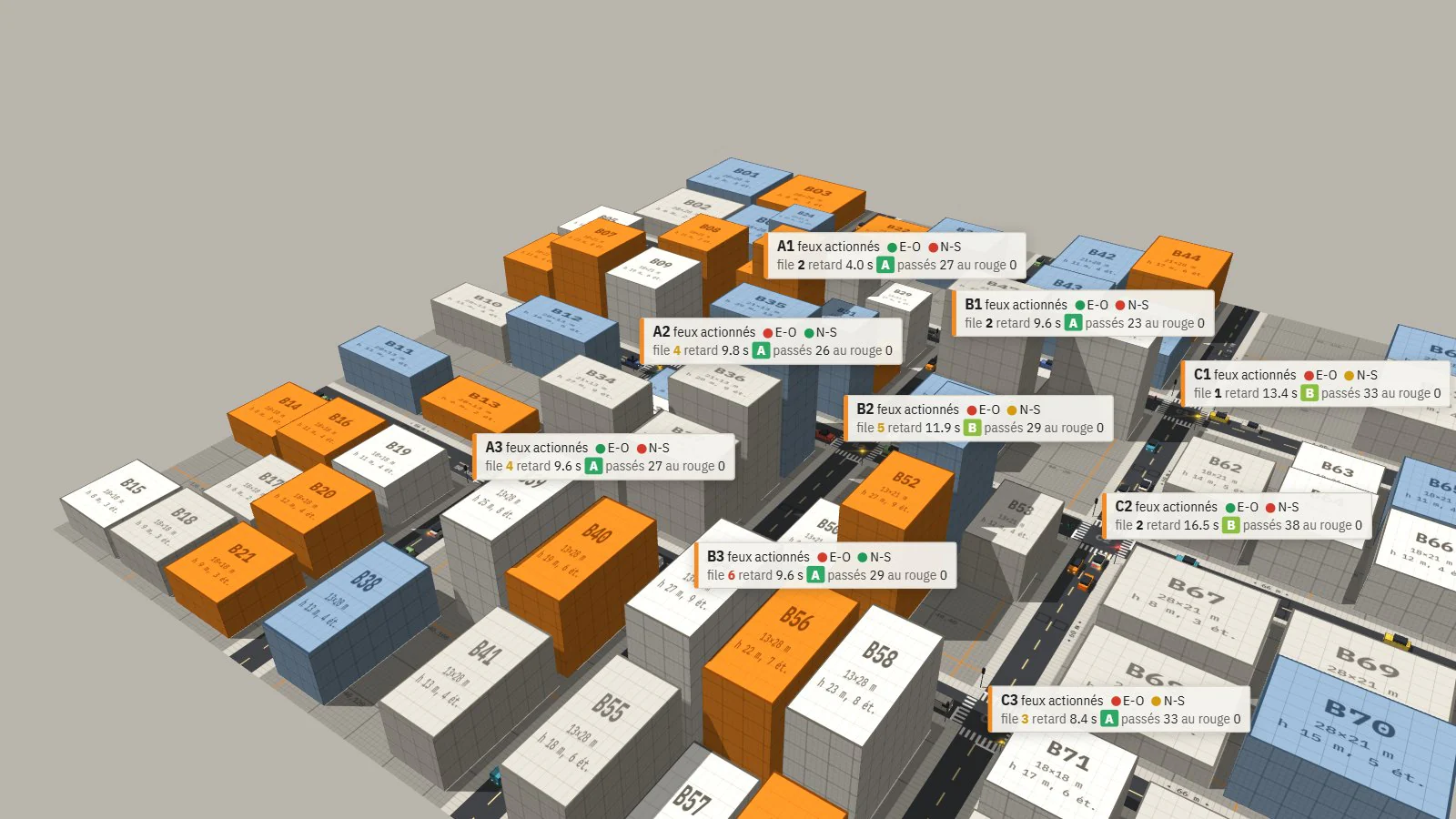
Webster coordination: every 5 min, a common cycle C₀ = (1.5 L + 5) / (1 − Y) computed from the loop flows, with a lost time L of 6 s per phase and a cycle bounded between 30 and 120 s; greens shared by load; offsets of the form a·column + b·row, chosen to maximise the total width of the green bands at 40 km/h in both directions. On this grid (60 m blocks, cycle of about 40 s), the optimum is a wave in one direction per axis. At 70 veh/min: control delay of 27.0 s against 28.4 s for the fixed-cycle green wave, CO₂ −4.5%.

Max-pressure: a phase’s pressure is the sum, over its requested movements, of the waiting vehicles minus the queue on their exit. A decision every 2 s, after a 12 s minimum green; the opposing phase takes green if its pressure exceeds the current phase’s by at least 3 vehicles. A lower threshold (6 s minimum green, switching at the slightest difference) costs more in phase changes than it gains: 39.5 s delay.

Log 04 / 10
Instrumentation
Vehicle inspector, heat map, sensors, levels of service, calibration.
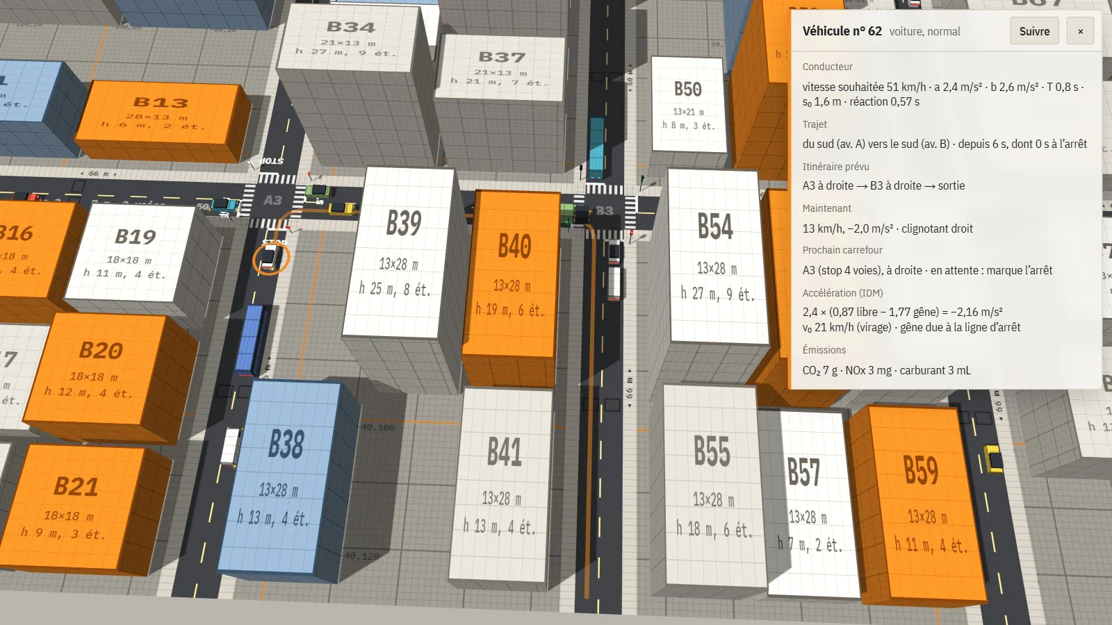
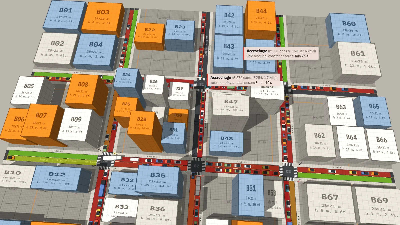
Inspector: clicking a vehicle opens its sheet, with driver profile and parameters, trip, planned route (drawn on the ground), intention and booking at the next junction or the reason it is waiting, the IDM acceleration terms and their cause, emissions. Heat map: each lane’s mean speed relative to its limit, over a sliding 20 s. The ?debug URL exposes the full state in the console.
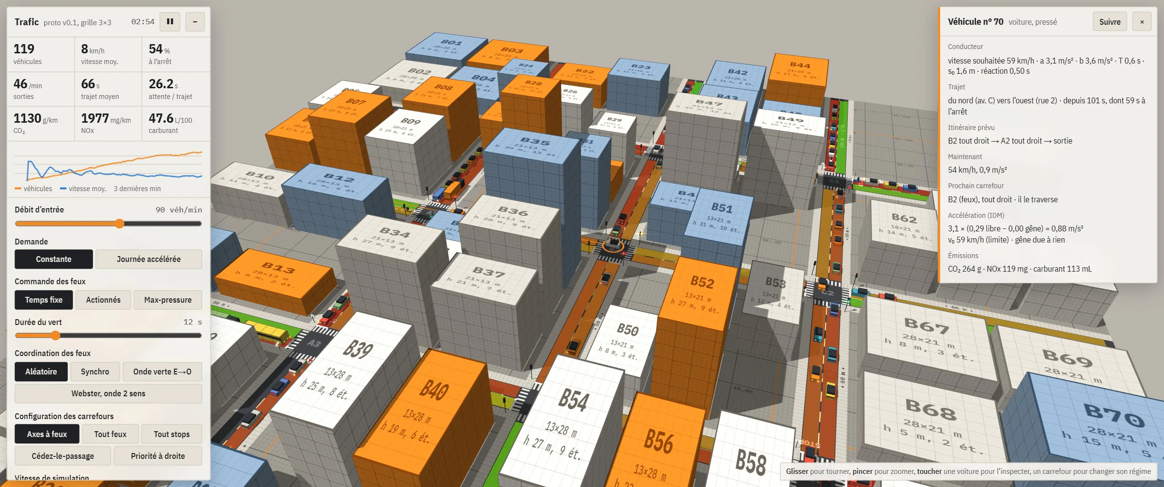
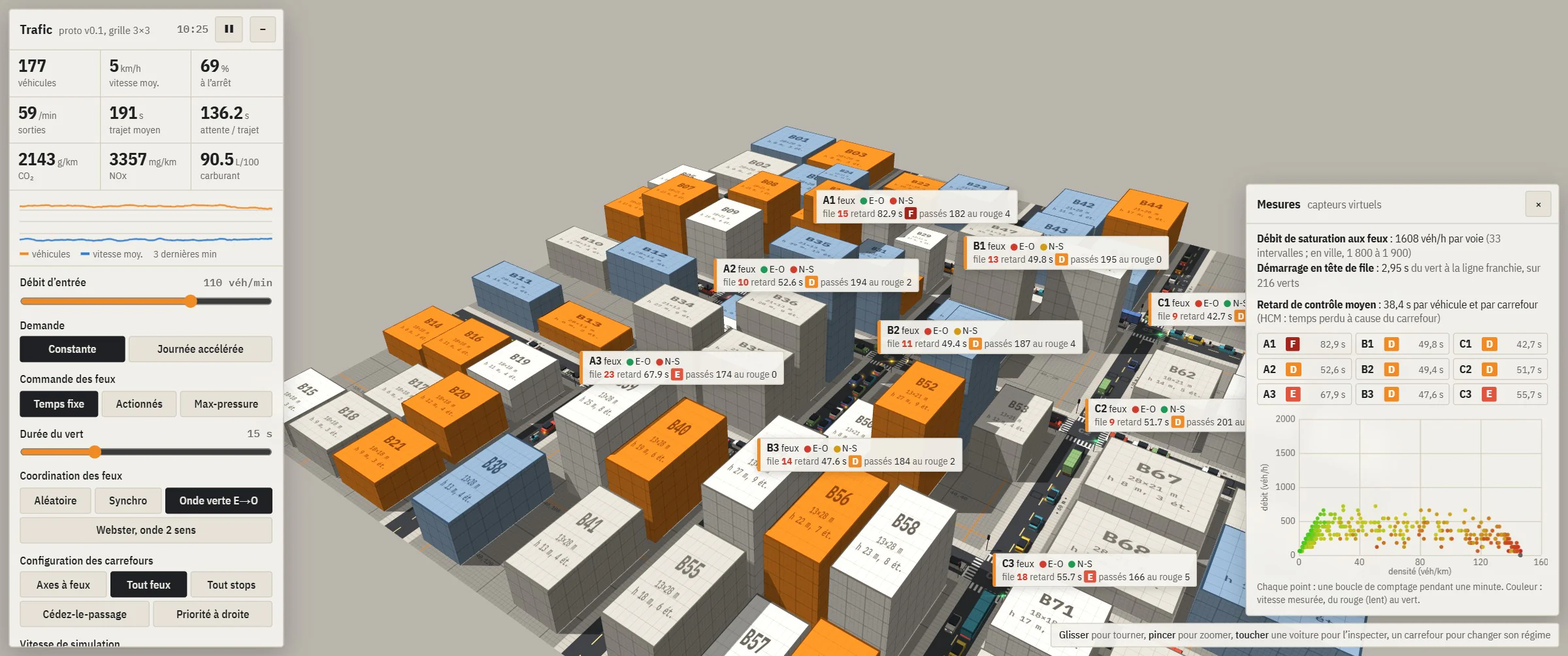
Sensors: a virtual counting loop in the middle of each lane (flow, occupancy, speed, aggregated per minute); control delay per vehicle and per junction, converted into a level of service A to F at HCM thresholds; saturation flow measured at signals from the 5th vehicle in a queue; flow-density diagram.
Calibration: the first measurement gave 1,250 veh/h per lane, against 1,800 to 1,900 observed in cities. Fixes: gap to the vehicle ahead underestimated by 0.7 m, junction anti-blocking rule too strict, IDM parameters brought back into the ranges published for urban driving. Side effect: waiting per trip −30 to −38%.
- 1,250
- Veh/h per lane, saturation flow before calibration.
- 1,824
- Veh/h per lane after calibration (± 49), cars only.
- 1,640
- Veh/h per lane with 7% trucks and buses, consistent with the HCM correction.
Log 05 / 10
Demand and fleet
Origin-destination matrix, shortest path, five vehicle types, emissions.
Routes: each vehicle gets a destination on entry, drawn from an origin-destination matrix, and takes the fastest path, in time at the speed limit plus 3 s per right turn and 8 s per left turn; random choice between paths within 1 s of the best. Resulting split: 58% straight, 22% right, 20% left. Accelerated-day mode (1 min = 1 h): peaks at 8 am and 5 pm, destinations leaning east in the morning and west in the evening.
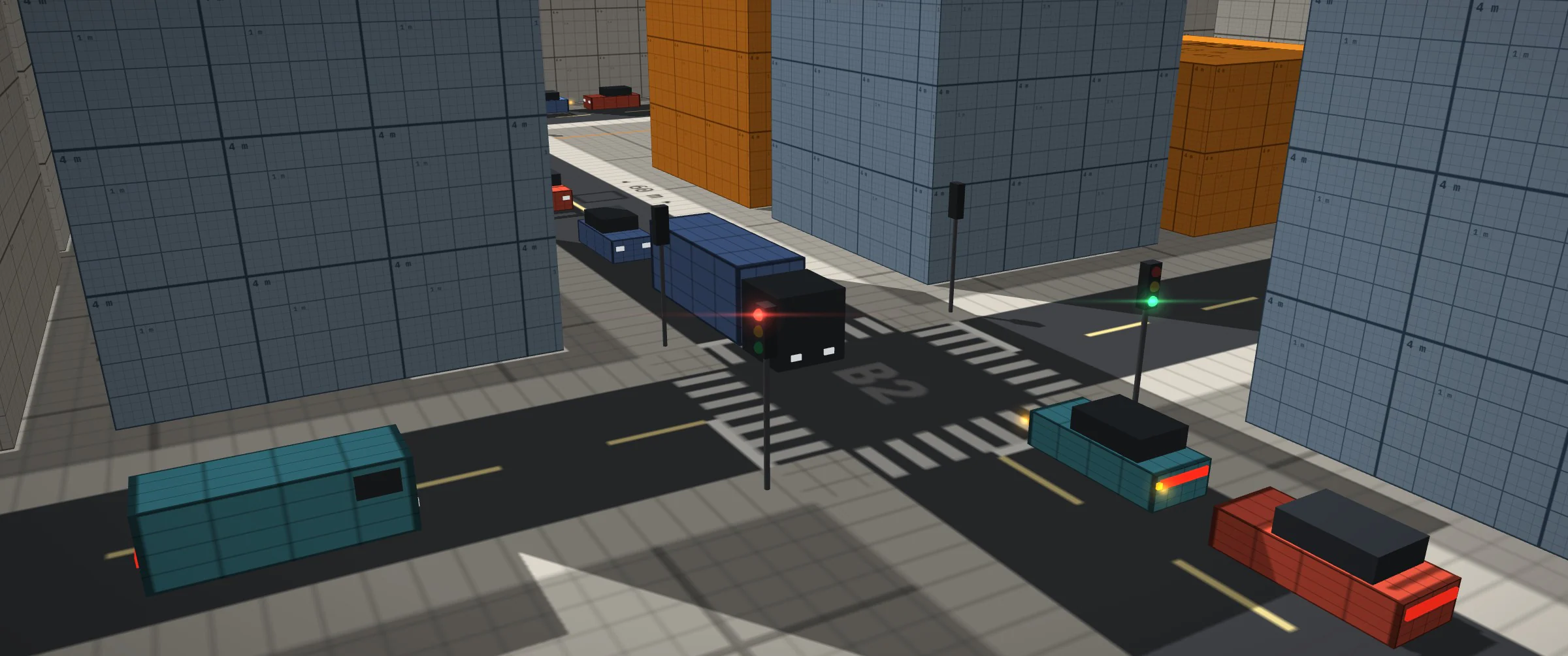
Fleet: cars 80%, vans 8%, trucks 4% (10 m), buses 3% (12 m), two-wheelers 5%. Each type has its own size, acceleration, braking, critical gap (+1 s for heavy vehicles) and emission class; the single length constant is gone from the engine. A heavy vehicle keeps its junction booking until its rear has left it. Validation: no gridlock over six seeds at 70, 110 and 140 veh/min; saturation flow of 1,643 veh/h on the green wave.
Emissions: CO₂, NOx and fuel computed at every step from speed and acceleration, with SUMO’s HBEFA3 coefficients and fuel cut-off when decelerating. Check at a steady 50 km/h: 168 g/km of CO₂ and 7.2 L/100 km (Euro 4 petrol). On the grid, averages (500 to 1,400 g/km) are dominated by idling; they are used to compare settings. For example, 30 zones on the outer axes: average speed −3%, trips +3%, CO₂ per kilometre −7%.
Log 06 / 10
Drivable vehicle
Bicycle dynamics, collisions, traffic rules, GPS and missions.
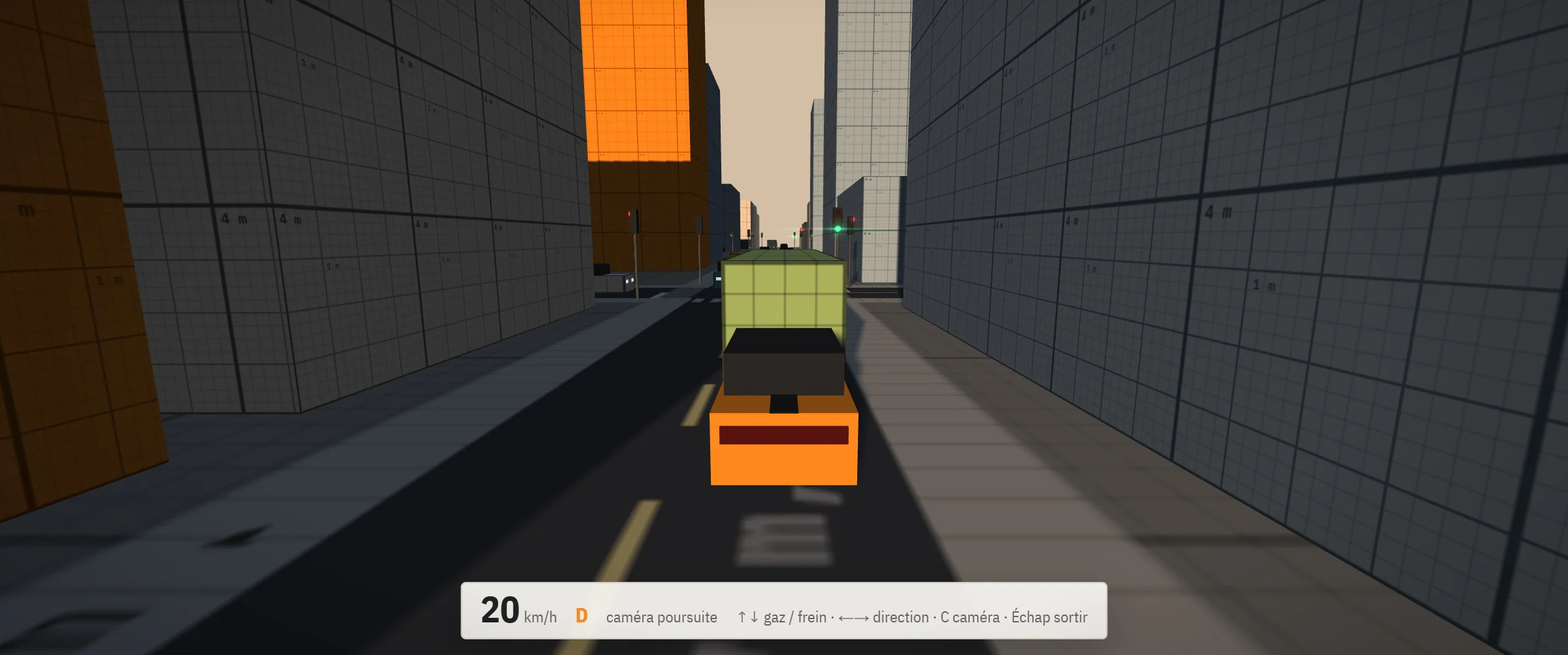
Dynamics: bicycle model with tyre grip; 1,300 kg, 2.6 m wheelbase, 75 kW, front-wheel drive; 0 to 100 km/h in 8.4 s, 50 to 0 km/h in 11 m; loss of grip when braking or accelerating in a bend. Keyboard or gamepad; chase, cockpit and free cameras.
Collisions: vehicles approximated by three circles along their axis, buildings by their boxes. Penetration resolved, then a rigid-body impulse: bounce, rotation depending on the point of impact, sliding along walls (friction 0.2). An AI vehicle that is hit absorbs the shock along its path and stops.
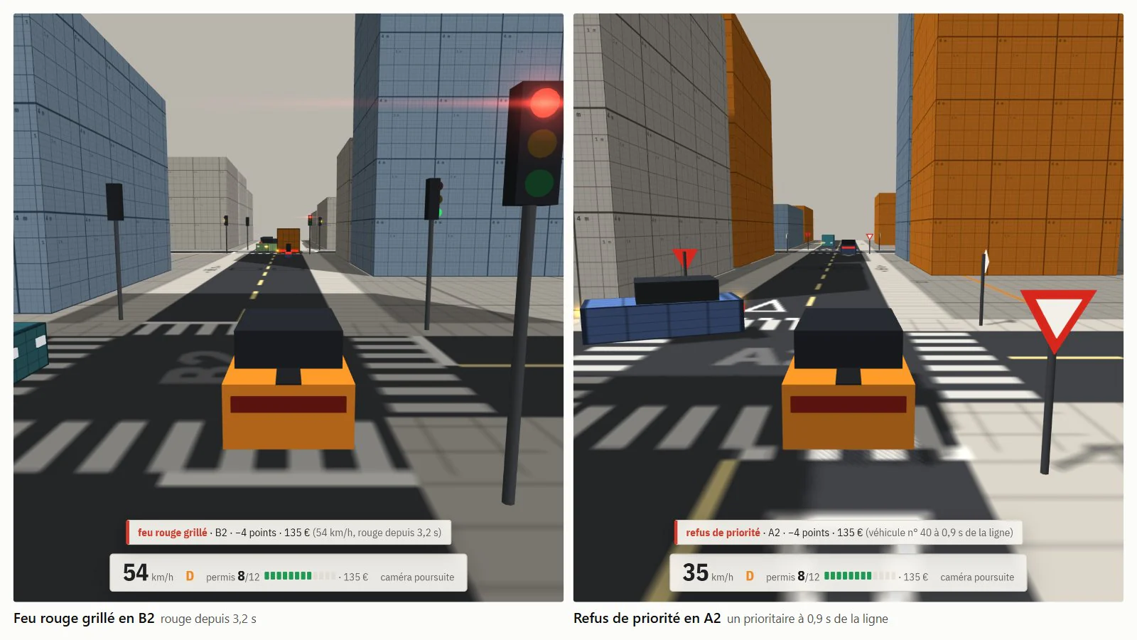
Traffic rules: 12-point licence, ANTAI scale. The player’s free position is attached at every step to the segment whose carriageway contains it and whose direction matches its heading (map matching); that segment gives the limit, the next junction and its regime. Line crossings are detected between two steps on the position of the vehicle’s front; speed is checked continuously, in whole km/h, with a 5 km/h margin deducted.
| Offence | Detection | Points |
|---|---|---|
| Red light | The front crosses the line on red. | 4 |
| Avoidable amber | When it came on, required braking v² / 2d below 4.5 m/s². | 4 |
| Rolled stop | No full stop (< 1 km/h) within the last 15 metres. | 4 |
| Failure to give way | Priority vehicle less than 3 s from the line, or already in the junction. | 4 |
| Speeding | Recorded speed = measured − 5 km/h, at the peak of the excess. | 0 to 6 |

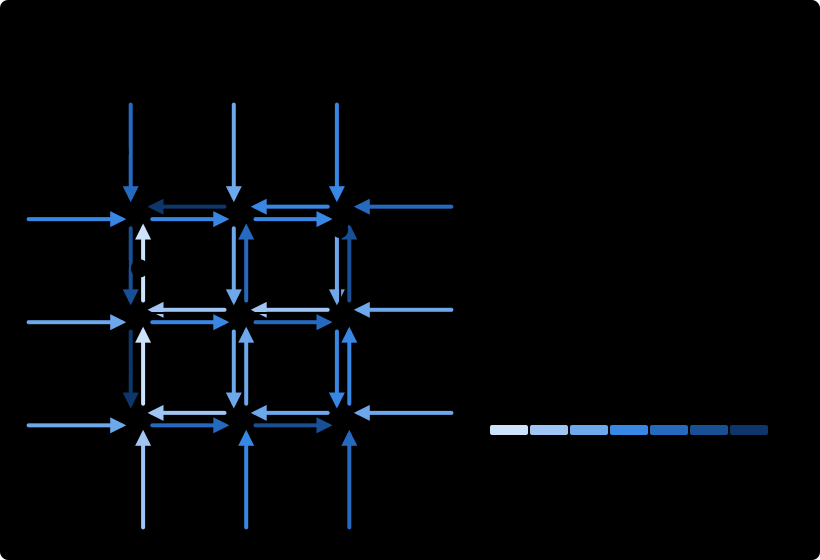
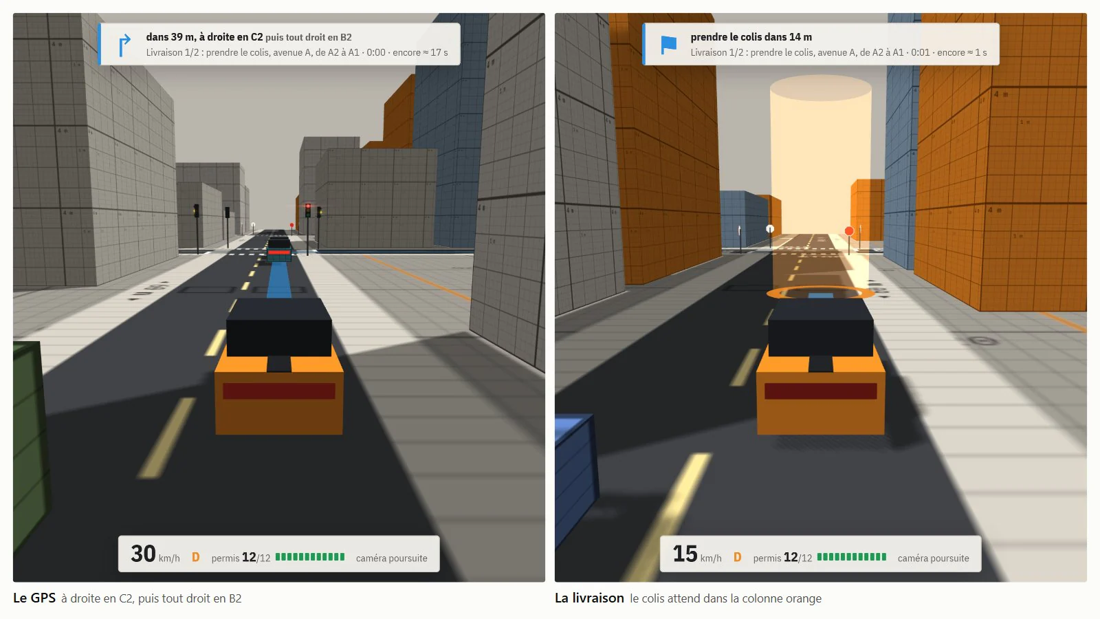
GPS: a graph whose nodes are the segments and whose edges are the allowed movements (no U-turns), with the same costs as the AI routes. The time remaining to the destination is computed for every segment, backwards (Bellman-Ford, a few passes over 48 segments); at each junction, guidance takes the branch that minimises turn + time remaining. A deviation from the route therefore needs no recomputation. The displayed ribbon is updated on segment changes and four times per second.
Missions: trip, delivery, time trial. Stops are drawn from a separate random stream, with no effect on traffic; a stop is validated within 6 m, below 1 m/s for 1 s; time trials are judged at 1, 1.2 and 1.5 times the estimated time, with a 10 s penalty per offence.
Log 07 / 10
Disruptions
Distraction and fender benders, weather and visibility, scheduled events.
Distraction (optional): inattention episodes while driving (one every 40 s on average, × 0.6 for a cautious driver, × 1.5 for a hurried one; lognormal duration, median 1.1 s, at most 4 s) and while stopped (after 2 s of waiting, one every 12 s, median 2.5 s, foot on the brake). During an episode, perception is frozen. The return to the road is triggered by a time-to-collision below a threshold with a 1.8 s median or by the vehicle ahead pulling away (4 m), then the reaction time applies.
Fender bender: contact at 1 m/s or more on the same segment. Both vehicles stop with hazard lights on for the duration of the accident report (median 2 min 30 s, 1 to 6 min) and block the lane; the queue upstream triggers route changes at the previous junctions.
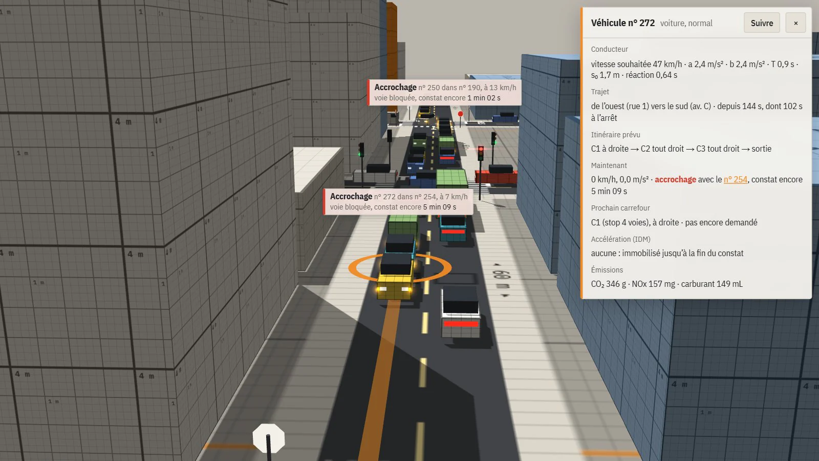
- 1.49 → 1.92 s
- Queue-head start-up, without then with distraction.
- 16.8 → 19.9 s
- Mean control delay.
- ≈ 3 / h
- Fender benders, deliberately above reality. Option off: bench identical bit for bit.
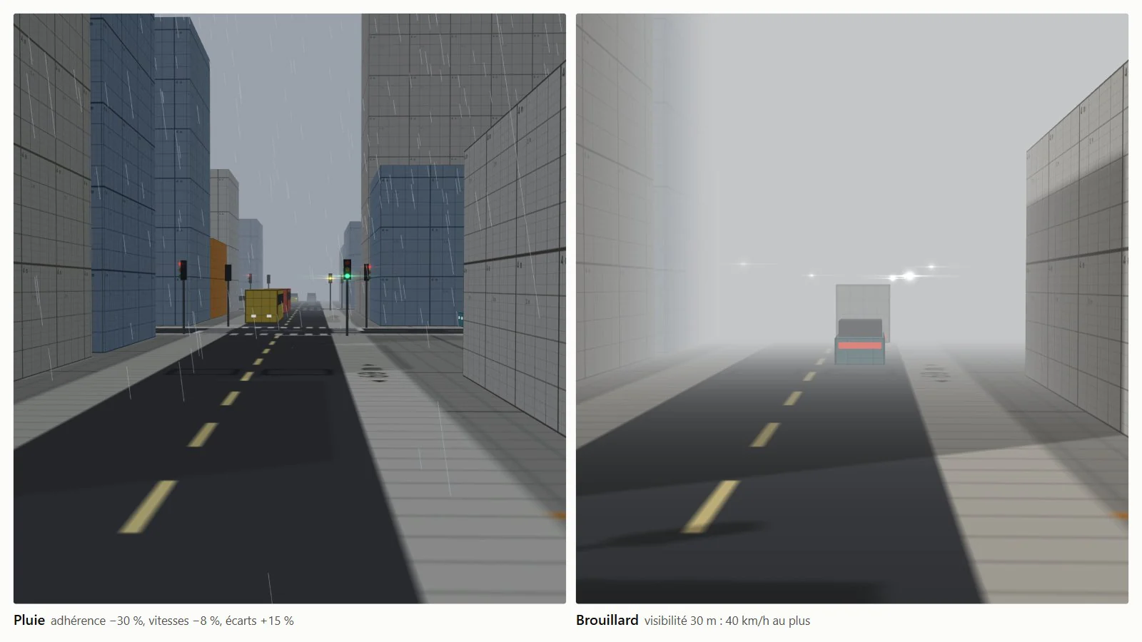
Weather: rain, fog and night act on every driver’s parameters, on top of their profile. Rain: grip × 0.7, speeds × 0.92, gaps × 1.15, acceleration × 0.9, comfortable braking × 0.85. Fog: 30 m visibility. Night: 80 m visibility. Grip bounds every braking (emergency, dilemma zone, player vehicle), and the desired speed is capped so the driver can stop within the visibility: Tr·v + v² / 2b ≤ visibility, i.e. 40 km/h at most in fog. In fair weather by day, every factor is 1 and the bench is unchanged bit for bit.

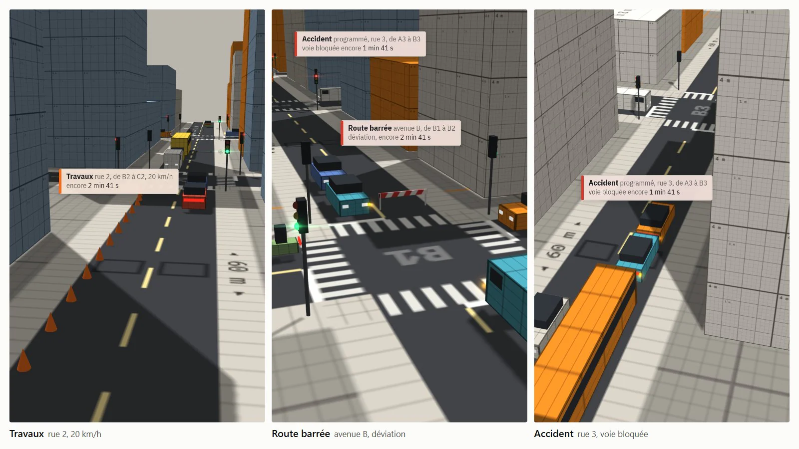
Events: roadworks (20 km/h over 32 m), closure and accident, scheduled per segment with a start time and duration. Each event changes the segment’s cost in the route computation shared with the GPS: infinite for a closure, the time lost for roadworks, a 90 s penalty for an accident. At every event start and end, the remaining times are recomputed; drivers who have not yet booked their next junction choose their branch again, and those whose exit becomes unreachable change it. Traffic diversions follow from these costs alone.


Log 08 / 10
Architecture and data
Engine without global state, versioned JSON formats, curved segments.
The engine (src/sim/) is pure JavaScript, with no three.js and no DOM: it runs under Node for the bench and the figures, and in the browser for the app. Its state lives in a world object created by createWorld(): settings, network, traffic, sensors, signal coordination, events, weather. Modules are factories that receive a world and read its parts under their usual names; the functions’ code did not change. Rendering and UI read the app’s world through src/world.js. The refactor keeps the fingerprints of the 18 scenarios and the figures byte for byte.


Network format: a JSON file of nodes (position in metres; regime and priority axis for a junction, nothing for an end point) and streets (name, speed limit, sequence of nodes). The engine derives the segments (one per direction, shortened by 6 m for the stop line), turning curves, entries, exits and remaining-time tables. The scenario format adds settings, signal plans, entry and exit weights, and events. The loader reproduces the creation order of the old hard-coded grid: same numbering, same draws, identical fingerprints.
{
  "format": "trafic-scenario",
  "version": 1,
  "network": "boulevard",
  "settings": { "preset": "mixed", "control": "fixed", "coord": "plan", "rate": 24 },
  "plans": {
    "J1": { "green": [35, 16], "offset": 0 },
    "J2": { "green": [35, 16], "offset": 5 },
    "J3": { "green": [35, 16], "offset": 10 },
    "J4": { "green": [35, 16], "offset": 15 }
  },
  "demand": { "entries": { "O": 4, "E": 4 }, "exits": { "O": 8, "E": 8 } }
}
Test network: a 252 m east-west boulevard with four signals, plan offset in 5 s steps (wave at 43 km/h). Eastbound, a 36 s green band per cycle and 42% of trips without a stop; westbound, 6 s and 5%.

Validation: both formats are versioned; npm run datas checks a file before anything is built and lists all its errors, one per mistake, including what the engine version cannot drive yet.
✗ casse.json
  Réseau « Réseau cassé » : 9 erreurs
    - rue « rue haute » : nœud inconnu « X9 »
    - rue « rue basse » : vitesse limite 200 hors de 10 à 130 km/h
    - rue « rue basse », de J1 à J2 : ce tronçon existe déjà
    - rue « impasse », de J1 à J3 : 8 m entre lignes d’arrêt, il en faut au moins 20
    - il faut au moins deux extrémités, pour entrer et sortir (1 trouvée)
Curved segments (format v2): shape points, joined by circular arcs tangent to both stretches, with the given radius. Vehicles are still located by their arc length s: distances, queues, loops and roadwork zones are unchanged, only the s → position conversion changes (inverse accurate to 3 × 10⁻¹⁴ m, used for the player’s vehicle). The twenty or so reads of “segment direction” now distinguish arrival and departure direction. Comfort speed √(2.5 R), targeted 1 s before the bend to make up for the IDM’s lag in reaching its desired speed; time lost in bends goes into route costs and out of control delay.


Log 09 / 10
Rendering
three.js r128: interpolation, vehicle lights, procedural asphalt.
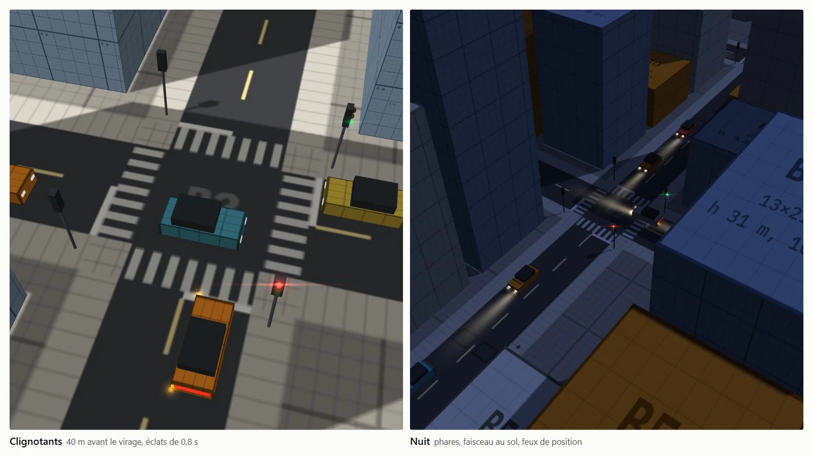
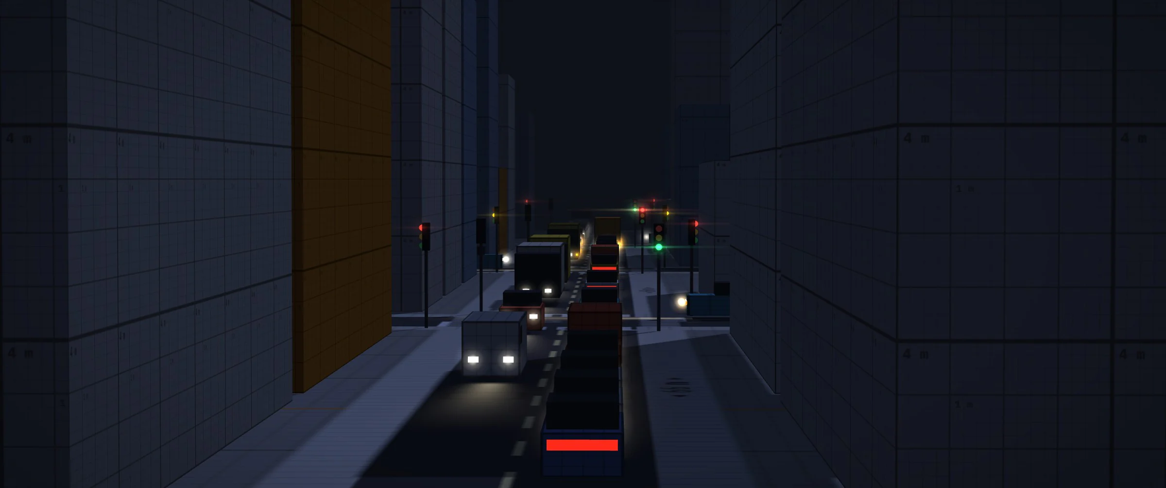
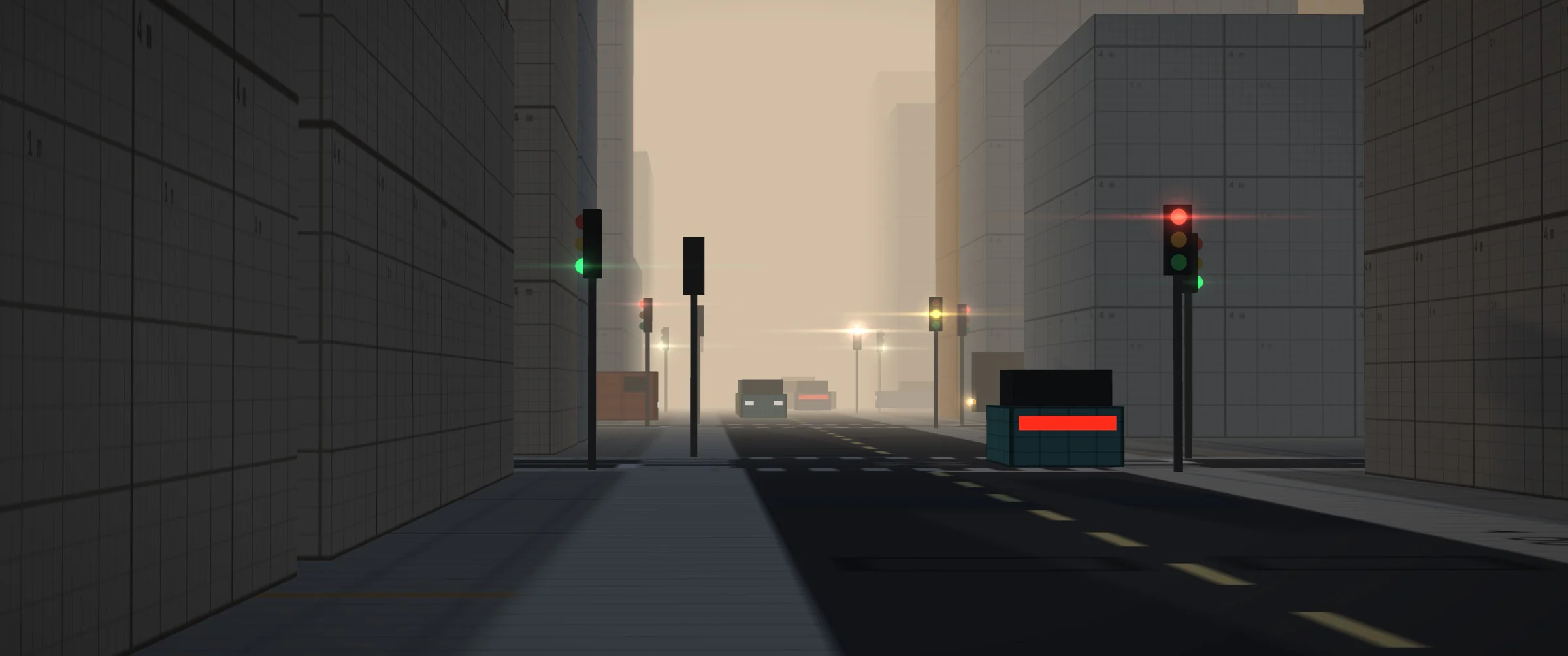
Rendering reads the simulation state without modifying it. Vehicles as InstancedMesh; position and heading interpolated between the last two steps, with one step (33 ms) of latency, for smooth motion at 60 Hz and above. Brake lights when braking, indicators 40 m before the turn (intention carried by the simulation), hazard lights; at night, headlights with a beam on the ground, side lights and halos at metric scale. Building shadows fall on the vehicles.
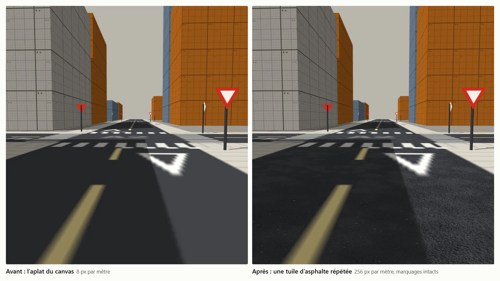
Asphalt: the ground is a 2,048 px canvas texture for 256 m (8 px/m, 28 px per lane), not enough at eye level; the grain of asphalt would need 256 px/m. A 4 m tile (1,024 px) repeated 64 times in each direction provides that grain. It comes from a procedural MaterialCraft graph (binder, 1 to 2 cm chippings, larger stones, undulation and wear), periodic by construction: every generator has a whole-number scale over the tile. It contains no identifiable pattern, so the repetition does not show.
 Fig. 35 · basecolor
 Fig. 36 · normal
4 m tile, colour and normals, exported from the graph (asphalte.mcraft, 2 kB).
Ground shader: asphalt is only applied to bare road surface, detected by the distance to its colour in the canvas (blended between 0.03 and 0.08), so markings stay intact. The tile modulates the colour instead of replacing it: colour × tile / tile average, the average being read from the last mipmap level; from a distance, the original tint is preserved. The normal map is read in tile coordinates by replacing three.js’s normal_fragment_maps block, with a console warning if the targeted block changes. The ground moves from Lambert (per-vertex lighting) to Phong without specular (per-pixel lighting). Cost: three extra texture reads per ground pixel.
Log 10 / 10
Roadmap
28 of 50 features done; tier 1 complete, tier 2 up to #28.
Fifty features in four tiers, ranked by size (S to XL) then by value, with dependencies respected. The app reads ROADMAP.md and shows progress on its #roadmap page: done, in progress, ready to start.
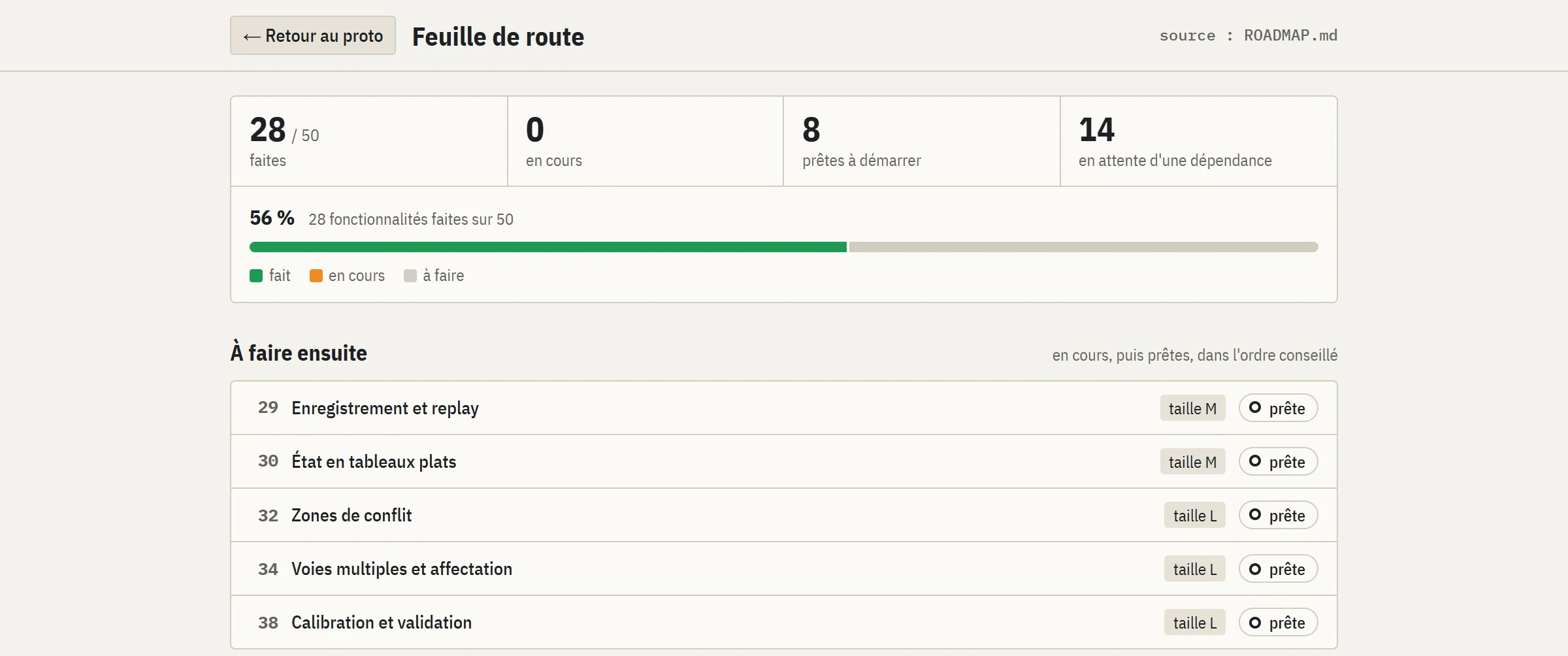
Rest of tier 2: recording and replay from the seed and inputs (#29), state in typed arrays read without copying by the renderer (#30), simulation in a Web Worker (#31). Main tier 3 projects:
- 01
#32 Conflict zones
Conflict points per pair of paths; booking only the points crossed instead of the whole junction.
- 02
#33 Player in traffic
The AI drivers perceive the player’s vehicle, its indicators and merges; the player books junctions like they do.
- 03
#34–37 Multiple lanes
Several lanes each way with allowed movements, MOBIL lane changes, positioning ahead of time for the route, merges and zipper merging.
- 04
#38 Calibration
Fitting to real counts and travel times, comparison with SUMO on the same scenarios.
Then: junctions with any number of arms at any angle, multi-phase signal plans (NEMA), dynamic assignment to Wardrop equilibrium, steering kinematics for the AI, parking, public transport, cyclists, a network editor, roundabouts, emergency vehicles. Tier 4: OpenStreetMap import (an extract of about 1.65 × 1 km near Nagoya is already in the repository) and pedestrians following a social force model (Helbing and Molnár, 1995).
- Project
- Personal, in progress
- Version
- Prototype 0.1, #28, 5 November 2026
- Models
- IDM · HDM · HCM · Webster · Max-pressure · HBEFA3
- Emissions
- HBEFA3 coefficients from SUMO (© DLR, EPL 2.0)
- JavaScript
- three.js r128
- GLSL
- Vite
- Node
- playwright-core
- SVG
- JSON
- MaterialCraft


